총 고객 100명인데, 휴면 고객이 50명이라면?
업데이트:
Predict Customer Churn
- Start: 20.06.24
- End: 20.07.22
고객 데이터에 관심이 많다. 특히 고객 이탈에 대해 공부를 해보고 싶었는데, Kaggle에 공개된 데이터셋이 존재했다.
- 데이터셋: 캐글 데이터셋
About project (TMI)

- 서비스에서 가장 중요한 것이 뭐냐고 묻는다면 나는 고객이라고 답할것이다. 고객이 없다면 서비스의 존재 이유가 사라지기 때문이다.
- 고객은 다음과 같이 크게 세 분류로 나눌 수 있을것이다.
- 신규 고객: 브랜드 경험과 이해도가 적다. 애정 또한 낮다.
- 충성 고객: 브랜드에 긍정적인 경험을 가지고있고, 서비스를 꾸준히 이용한다.
- 이탈 고객: 우리 서비스를 이용했었지만 이제 떠난 고객이다. 이탈을 영어로는 churn 이라고 한다.
- 서비스를 성공시키기 위해서는, 1) 신규 고객을 2) 충성 고객으로 만드는 것이 중요하다.
- 또한 3) 이탈 고객이 되지 않도록 방지하는 것 또한 매우 중요하다. (이번 프로젝트는 이 요소에 중점을 둔다.)
- 고객은 다음과 같이 크게 세 분류로 나눌 수 있을것이다.
- e-커머스에서 이탈 고객 방지 프로젝트를 해보며 느낀 점은,
- 이탈할 것이라고 예상되는 고객 리스트가 있다면,
- 그들이 이탈하지 않도록 방지할 수 있고,
- 서비스를 더 성장시킬 수 있겠다는 것이다.
- 머신러닝을 공부하다보니 과거에 예측하지 못했던 부분들을 머신러닝 모델을 통해 가능하겠다는 생각이 들었다. (분류 문제로)
- 실제로 이탈 고객을 예측하는 모델을 만들어보기 위해 데이터를 찾다가
- 캐글에서 churn 여부가 기재된 고객 데이터를 찾게 되었다.
- 이탈 예정인 고객을 분류하는 모델을 실제로 만들어보자.
목차
1. 데이터 불러오기
import pandas as pd
pd.set_option('display.max_columns', 30)
import numpy as np
import matplotlib.pyplot as plt
plt.style.use('seaborn-whitegrid')
import seaborn as sns
import warnings
warnings.filterwarnings('ignore')
from sklearn.model_selection import train_test_split
import missingno as msno
from tqdm import tqdm_notebook
plt.rc('font', size=13)
plt.rc('font', family='NanumGothic')
df = pd.read_csv('source/Telco_Customer/Telco_Customer_Churn.csv')
df.shape
(7043, 21)
df.info()
<class 'pandas.core.frame.DataFrame'>
RangeIndex: 7043 entries, 0 to 7042
Data columns (total 21 columns):
customerID          7043 non-null object
gender              7043 non-null object
SeniorCitizen       7043 non-null int64
Partner             7043 non-null object
Dependents          7043 non-null object
tenure              7043 non-null int64
PhoneService        7043 non-null object
MultipleLines       7043 non-null object
InternetService     7043 non-null object
OnlineSecurity      7043 non-null object
OnlineBackup        7043 non-null object
DeviceProtection    7043 non-null object
TechSupport         7043 non-null object
StreamingTV         7043 non-null object
StreamingMovies     7043 non-null object
Contract            7043 non-null object
PaperlessBilling    7043 non-null object
PaymentMethod       7043 non-null object
MonthlyCharges      7043 non-null float64
TotalCharges        7043 non-null object
Churn               7043 non-null object
dtypes: float64(1), int64(2), object(18)
memory usage: 1.1+ MB
df.head(3)
| customerID | gender | SeniorCitizen | Partner | Dependents | tenure | PhoneService | MultipleLines | InternetService | OnlineSecurity | OnlineBackup | DeviceProtection | TechSupport | StreamingTV | StreamingMovies | Contract | PaperlessBilling | PaymentMethod | MonthlyCharges | TotalCharges | Churn | |
|---|---|---|---|---|---|---|---|---|---|---|---|---|---|---|---|---|---|---|---|---|---|
| 0 | 7590-VHVEG | Female | 0 | Yes | No | 1 | No | No phone service | DSL | No | Yes | No | No | No | No | Month-to-month | Yes | Electronic check | 29.85 | 29.85 | No |
| 1 | 5575-GNVDE | Male | 0 | No | No | 34 | Yes | No | DSL | Yes | No | Yes | No | No | No | One year | No | Mailed check | 56.95 | 1889.5 | No |
| 2 | 3668-QPYBK | Male | 0 | No | No | 2 | Yes | No | DSL | Yes | Yes | No | No | No | No | Month-to-month | Yes | Mailed check | 53.85 | 108.15 | Yes |
df.tail(3)
| customerID | gender | SeniorCitizen | Partner | Dependents | tenure | PhoneService | MultipleLines | InternetService | OnlineSecurity | OnlineBackup | DeviceProtection | TechSupport | StreamingTV | StreamingMovies | Contract | PaperlessBilling | PaymentMethod | MonthlyCharges | TotalCharges | Churn | |
|---|---|---|---|---|---|---|---|---|---|---|---|---|---|---|---|---|---|---|---|---|---|
| 7040 | 4801-JZAZL | Female | 0 | Yes | Yes | 11 | No | No phone service | DSL | Yes | No | No | No | No | No | Month-to-month | Yes | Electronic check | 29.60 | 346.45 | No |
| 7041 | 8361-LTMKD | Male | 1 | Yes | No | 4 | Yes | Yes | Fiber optic | No | No | No | No | No | No | Month-to-month | Yes | Mailed check | 74.40 | 306.6 | Yes |
| 7042 | 3186-AJIEK | Male | 0 | No | No | 66 | Yes | No | Fiber optic | Yes | No | Yes | Yes | Yes | Yes | Two year | Yes | Bank transfer (automatic) | 105.65 | 6844.5 | No |
- object 형식의 컬럼이 많은데, 대부분 No, Yes 형식의 binary text가 많다.
- 이 컬럼들은 전처리 시 [0, 1]로 변경하자.
- 그리고, 컬럼명이 어떤 것은 카멜표기법이고, 어떤것은 그냥 소문자 표기법이다.
- 오타도 줄일 겸, 모두 소문자로 컬럼명을 변경해버리자.
2. 데이터 전처리
2.1 컬럼명 변경
- 소문자로 변경하자
col_lower = [col.lower() for col in df.columns]
col_lower
['customerid',
 'gender',
 'seniorcitizen',
 'partner',
 'dependents',
 'tenure',
 'phoneservice',
 'multiplelines',
 'internetservice',
 'onlinesecurity',
 'onlinebackup',
 'deviceprotection',
 'techsupport',
 'streamingtv',
 'streamingmovies',
 'contract',
 'paperlessbilling',
 'paymentmethod',
 'monthlycharges',
 'totalcharges',
 'churn']
df.columns = col_lower
df.columns
Index(['customerid', 'gender', 'seniorcitizen', 'partner', 'dependents',
       'tenure', 'phoneservice', 'multiplelines', 'internetservice',
       'onlinesecurity', 'onlinebackup', 'deviceprotection', 'techsupport',
       'streamingtv', 'streamingmovies', 'contract', 'paperlessbilling',
       'paymentmethod', 'monthlycharges', 'totalcharges', 'churn'],
      dtype='object')
2.2 이진 텍스트 데이터 숫자로 변경
df.head()
| customerid | gender | seniorcitizen | partner | dependents | tenure | phoneservice | multiplelines | internetservice | onlinesecurity | onlinebackup | deviceprotection | techsupport | streamingtv | streamingmovies | contract | paperlessbilling | paymentmethod | monthlycharges | totalcharges | churn | |
|---|---|---|---|---|---|---|---|---|---|---|---|---|---|---|---|---|---|---|---|---|---|
| 0 | 7590-VHVEG | Female | 0 | Yes | No | 1 | No | No phone service | DSL | No | Yes | No | No | No | No | Month-to-month | Yes | Electronic check | 29.85 | 29.85 | No |
| 1 | 5575-GNVDE | Male | 0 | No | No | 34 | Yes | No | DSL | Yes | No | Yes | No | No | No | One year | No | Mailed check | 56.95 | 1889.5 | No |
| 2 | 3668-QPYBK | Male | 0 | No | No | 2 | Yes | No | DSL | Yes | Yes | No | No | No | No | Month-to-month | Yes | Mailed check | 53.85 | 108.15 | Yes |
| 3 | 7795-CFOCW | Male | 0 | No | No | 45 | No | No phone service | DSL | Yes | No | Yes | Yes | No | No | One year | No | Bank transfer (automatic) | 42.30 | 1840.75 | No |
| 4 | 9237-HQITU | Female | 0 | No | No | 2 | Yes | No | Fiber optic | No | No | No | No | No | No | Month-to-month | Yes | Electronic check | 70.70 | 151.65 | Yes |
cols = ['partner', 'dependents', 'phoneservice', 'multiplelines', 'onlinesecurity', 'onlinebackup',
        'deviceprotection', 'techsupport', 'streamingtv', 'streamingmovies',
        'paperlessbilling', 'churn']
for col in cols:
    print('{:<17}: {}'.format(col, df[col].unique()))
partner          : ['Yes' 'No']
dependents       : ['No' 'Yes']
phoneservice     : ['No' 'Yes']
multiplelines    : ['No phone service' 'No' 'Yes']
onlinesecurity   : ['No' 'Yes' 'No internet service']
onlinebackup     : ['Yes' 'No' 'No internet service']
deviceprotection : ['No' 'Yes' 'No internet service']
techsupport      : ['No' 'Yes' 'No internet service']
streamingtv      : ['No' 'Yes' 'No internet service']
streamingmovies  : ['No' 'Yes' 'No internet service']
paperlessbilling : ['Yes' 'No']
churn            : ['No' 'Yes']
- [‘No’ ‘Yes’ ‘No internet service’]는 [‘No’, ‘Yes’]로 변경해주고,
- No: 0과 Yes: 1로 변경해주자
for col in cols:
    df[col].replace({'No': 0,
                     'No internet service': 0,
                     'No phone service': 0,
                     'Yes': 1}, inplace=True)
df.head()
| customerid | gender | seniorcitizen | partner | dependents | tenure | phoneservice | multiplelines | internetservice | onlinesecurity | onlinebackup | deviceprotection | techsupport | streamingtv | streamingmovies | contract | paperlessbilling | paymentmethod | monthlycharges | totalcharges | churn | |
|---|---|---|---|---|---|---|---|---|---|---|---|---|---|---|---|---|---|---|---|---|---|
| 0 | 7590-VHVEG | Female | 0 | 1 | 0 | 1 | 0 | 0 | DSL | 0 | 1 | 0 | 0 | 0 | 0 | Month-to-month | 1 | Electronic check | 29.85 | 29.85 | 0 |
| 1 | 5575-GNVDE | Male | 0 | 0 | 0 | 34 | 1 | 0 | DSL | 1 | 0 | 1 | 0 | 0 | 0 | One year | 0 | Mailed check | 56.95 | 1889.5 | 0 |
| 2 | 3668-QPYBK | Male | 0 | 0 | 0 | 2 | 1 | 0 | DSL | 1 | 1 | 0 | 0 | 0 | 0 | Month-to-month | 1 | Mailed check | 53.85 | 108.15 | 1 |
| 3 | 7795-CFOCW | Male | 0 | 0 | 0 | 45 | 0 | 0 | DSL | 1 | 0 | 1 | 1 | 0 | 0 | One year | 0 | Bank transfer (automatic) | 42.30 | 1840.75 | 0 |
| 4 | 9237-HQITU | Female | 0 | 0 | 0 | 2 | 1 | 0 | Fiber optic | 0 | 0 | 0 | 0 | 0 | 0 | Month-to-month | 1 | Electronic check | 70.70 | 151.65 | 1 |
df.info()
<class 'pandas.core.frame.DataFrame'>
RangeIndex: 7043 entries, 0 to 7042
Data columns (total 21 columns):
customerid          7043 non-null object
gender              7043 non-null object
seniorcitizen       7043 non-null int64
partner             7043 non-null int64
dependents          7043 non-null int64
tenure              7043 non-null int64
phoneservice        7043 non-null int64
multiplelines       7043 non-null int64
internetservice     7043 non-null object
onlinesecurity      7043 non-null int64
onlinebackup        7043 non-null int64
deviceprotection    7043 non-null int64
techsupport         7043 non-null int64
streamingtv         7043 non-null int64
streamingmovies     7043 non-null int64
contract            7043 non-null object
paperlessbilling    7043 non-null int64
paymentmethod       7043 non-null object
monthlycharges      7043 non-null float64
totalcharges        7043 non-null object
churn               7043 non-null int64
dtypes: float64(1), int64(14), object(6)
memory usage: 1.1+ MB
2.3 Totalcharges 컬럼
- 해당 컬럼이 object로 되어있는 것을 보아, 컬럼 내 문자가 포함되어있나보다.
df.totalcharges.value_counts().sort_index()[:5]
          11
100.2      1
100.25     1
100.35     1
100.4      1
Name: totalcharges, dtype: int64
- 공백문자가 껴있다. 해당 레코드를 확인해보자.
df[df.totalcharges==' ']
| customerid | gender | seniorcitizen | partner | dependents | tenure | phoneservice | multiplelines | internetservice | onlinesecurity | onlinebackup | deviceprotection | techsupport | streamingtv | streamingmovies | contract | paperlessbilling | paymentmethod | monthlycharges | totalcharges | churn | |
|---|---|---|---|---|---|---|---|---|---|---|---|---|---|---|---|---|---|---|---|---|---|
| 488 | 4472-LVYGI | Female | 0 | 1 | 1 | 0 | 0 | 0 | DSL | 1 | 0 | 1 | 1 | 1 | 0 | Two year | 1 | Bank transfer (automatic) | 52.55 | 0 | |
| 753 | 3115-CZMZD | Male | 0 | 0 | 1 | 0 | 1 | 0 | No | 0 | 0 | 0 | 0 | 0 | 0 | Two year | 0 | Mailed check | 20.25 | 0 | |
| 936 | 5709-LVOEQ | Female | 0 | 1 | 1 | 0 | 1 | 0 | DSL | 1 | 1 | 1 | 0 | 1 | 1 | Two year | 0 | Mailed check | 80.85 | 0 | |
| 1082 | 4367-NUYAO | Male | 0 | 1 | 1 | 0 | 1 | 1 | No | 0 | 0 | 0 | 0 | 0 | 0 | Two year | 0 | Mailed check | 25.75 | 0 | |
| 1340 | 1371-DWPAZ | Female | 0 | 1 | 1 | 0 | 0 | 0 | DSL | 1 | 1 | 1 | 1 | 1 | 0 | Two year | 0 | Credit card (automatic) | 56.05 | 0 | |
| 3331 | 7644-OMVMY | Male | 0 | 1 | 1 | 0 | 1 | 0 | No | 0 | 0 | 0 | 0 | 0 | 0 | Two year | 0 | Mailed check | 19.85 | 0 | |
| 3826 | 3213-VVOLG | Male | 0 | 1 | 1 | 0 | 1 | 1 | No | 0 | 0 | 0 | 0 | 0 | 0 | Two year | 0 | Mailed check | 25.35 | 0 | |
| 4380 | 2520-SGTTA | Female | 0 | 1 | 1 | 0 | 1 | 0 | No | 0 | 0 | 0 | 0 | 0 | 0 | Two year | 0 | Mailed check | 20.00 | 0 | |
| 5218 | 2923-ARZLG | Male | 0 | 1 | 1 | 0 | 1 | 0 | No | 0 | 0 | 0 | 0 | 0 | 0 | One year | 1 | Mailed check | 19.70 | 0 | |
| 6670 | 4075-WKNIU | Female | 0 | 1 | 1 | 0 | 1 | 1 | DSL | 0 | 1 | 1 | 1 | 1 | 0 | Two year | 0 | Mailed check | 73.35 | 0 | |
| 6754 | 2775-SEFEE | Male | 0 | 0 | 1 | 0 | 1 | 1 | DSL | 1 | 1 | 0 | 1 | 0 | 0 | Two year | 1 | Bank transfer (automatic) | 61.90 | 0 |
- 총 11개로 적기때문에, 해당 레코드들은 삭제해주자.
df = df[df['totalcharges'] != ' ']
df.totalcharges = df.totalcharges.astype('float')
df.info()
<class 'pandas.core.frame.DataFrame'>
Int64Index: 7032 entries, 0 to 7042
Data columns (total 21 columns):
customerid          7032 non-null object
gender              7032 non-null object
seniorcitizen       7032 non-null int64
partner             7032 non-null int64
dependents          7032 non-null int64
tenure              7032 non-null int64
phoneservice        7032 non-null int64
multiplelines       7032 non-null int64
internetservice     7032 non-null object
onlinesecurity      7032 non-null int64
onlinebackup        7032 non-null int64
deviceprotection    7032 non-null int64
techsupport         7032 non-null int64
streamingtv         7032 non-null int64
streamingmovies     7032 non-null int64
contract            7032 non-null object
paperlessbilling    7032 non-null int64
paymentmethod       7032 non-null object
monthlycharges      7032 non-null float64
totalcharges        7032 non-null float64
churn               7032 non-null int64
dtypes: float64(2), int64(14), object(5)
memory usage: 1.2+ MB
- 처리 완료!
3. 데이터 살펴보기
- EDA전에, test 세트는 미리 구분하여 들여다보지 않기
df_train, df_test = train_test_split(df)
print(df_train.shape, df_test.shape)
(5274, 21) (1758, 21)
df_train.head()
| customerid | gender | seniorcitizen | partner | dependents | tenure | phoneservice | multiplelines | internetservice | onlinesecurity | onlinebackup | deviceprotection | techsupport | streamingtv | streamingmovies | contract | paperlessbilling | paymentmethod | monthlycharges | totalcharges | churn | |
|---|---|---|---|---|---|---|---|---|---|---|---|---|---|---|---|---|---|---|---|---|---|
| 4101 | 9780-FKVVF | Male | 0 | 0 | 0 | 6 | 1 | 0 | DSL | 1 | 0 | 0 | 0 | 0 | 1 | Month-to-month | 1 | Bank transfer (automatic) | 59.15 | 336.70 | 0 |
| 3489 | 0975-UYDTX | Female | 0 | 1 | 0 | 26 | 1 | 1 | DSL | 1 | 1 | 1 | 1 | 1 | 1 | One year | 1 | Credit card (automatic) | 90.10 | 2312.55 | 0 |
| 4219 | 5176-LDKUH | Female | 0 | 0 | 0 | 48 | 1 | 0 | Fiber optic | 0 | 1 | 0 | 0 | 0 | 0 | One year | 0 | Electronic check | 75.15 | 3772.65 | 0 |
| 5091 | 2606-RMDHZ | Male | 0 | 0 | 0 | 6 | 0 | 0 | DSL | 0 | 1 | 0 | 0 | 0 | 0 | Month-to-month | 1 | Credit card (automatic) | 30.50 | 208.70 | 1 |
| 5398 | 3936-QQFLL | Male | 0 | 0 | 0 | 2 | 1 | 0 | No | 0 | 0 | 0 | 0 | 0 | 0 | Month-to-month | 0 | Mailed check | 19.75 | 39.30 | 0 |
3.1 Churn
sns.countplot(df_train.churn)
<matplotlib.axes._subplots.AxesSubplot at 0x114ef1f2388>

print(df_train.churn.value_counts())
print('이탈 고객 비율: {:.2f}%'.format(df_train.churn.mean()*100))
df_train.churn.value_counts().plot('pie')
plt.show()
0    3884
1    1390
Name: churn, dtype: int64
이탈 고객 비율: 26.36%

- 이탈(churn)에 해당하는 레코드는 26%다.
- 이탈과 다른 특성들은 어떤 관계를 가지는지 살펴보자.
3.2 Gender
df_male = df_train[df_train.gender=='Male']
df_female = df_train[df_train.gender=='Female']

f, ax = plt.subplots(1, 2, figsize=(13, 7))
sns.countplot(df_train.gender, ax=ax[0])
ax[0].set_title('성별에 따른 고객 수')
sns.barplot('gender', 'churn', data=df_train, ax=ax[1])
ax[1].set_title('성별에 따른 churn 비율')
ax[1].set_ylim(0, 0.5)
print('Male ratio: {:.2f}%, Female ratio: {:.2f}%'.format(len(df_male) / len(df_train)*100,
                                                          len(df_female) / len(df_train)*100))
Male ratio: 50.32%, Female ratio: 49.68%

- 데이터셋 내 성비는 밸런스가 잘 맞는다.
- 성별에 따라 churn 비율의 차이는 또한 적다.
3.3 Demographic
- seniorcitizen, partner, dependents
def cplot(data, col, ax):
    sns.countplot(data[col], ax=ax)
    ax.set_title('{} ({:.2f}%)'.format(col, data[col].mean()*100))
f, ax = plt.subplots(1, 3, figsize=(20, 5))
cplot(df_train, 'seniorcitizen', ax[0])
cplot(df_train, 'partner', ax[1])
cplot(df_train, 'dependents', ax[2])
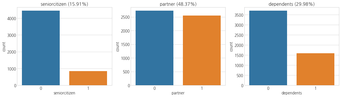
- 시니어의 비율은 약 16%를 차지하고,
- 배우자가 있는 사람은 48%,
- 자식이 있는 곳은 30%를 차지한다.
- 이제 여기에 churn을 함께 살펴보자.
def churnplot(data, col, ax):
    sns.countplot(col, hue='churn', data=data, ax=ax)
    ax.set_title('{} (0: {:.2f}%, 1: {:.2f}%)'.format(
    col,
    data[data[col] == 0].churn.mean()*100,
    data[data[col] == 1].churn.mean()*100))
f, ax = plt.subplots(1, 3, figsize=(20, 5))
churnplot(df_train, 'seniorcitizen', ax[0])
churnplot(df_train, 'partner', ax[1])
churnplot(df_train, 'dependents', ax[2])
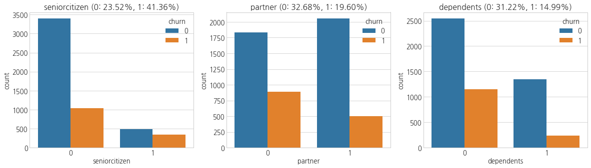
- 시니어일 경우, churn rate가 높다.
- 배우자나 자식이 있는 경우에는 churn rate가 상대적으로 낮다.
3.4 Tenure
- 계약 기간과 chunrate간의 관계를 파악해보자.
df_train.head()
| customerid | gender | seniorcitizen | partner | dependents | tenure | phoneservice | multiplelines | internetservice | onlinesecurity | onlinebackup | deviceprotection | techsupport | streamingtv | streamingmovies | contract | paperlessbilling | paymentmethod | monthlycharges | totalcharges | churn | |
|---|---|---|---|---|---|---|---|---|---|---|---|---|---|---|---|---|---|---|---|---|---|
| 4101 | 9780-FKVVF | Male | 0 | 0 | 0 | 6 | 1 | 0 | DSL | 1 | 0 | 0 | 0 | 0 | 1 | Month-to-month | 1 | Bank transfer (automatic) | 59.15 | 336.70 | 0 |
| 3489 | 0975-UYDTX | Female | 0 | 1 | 0 | 26 | 1 | 1 | DSL | 1 | 1 | 1 | 1 | 1 | 1 | One year | 1 | Credit card (automatic) | 90.10 | 2312.55 | 0 |
| 4219 | 5176-LDKUH | Female | 0 | 0 | 0 | 48 | 1 | 0 | Fiber optic | 0 | 1 | 0 | 0 | 0 | 0 | One year | 0 | Electronic check | 75.15 | 3772.65 | 0 |
| 5091 | 2606-RMDHZ | Male | 0 | 0 | 0 | 6 | 0 | 0 | DSL | 0 | 1 | 0 | 0 | 0 | 0 | Month-to-month | 1 | Credit card (automatic) | 30.50 | 208.70 | 1 |
| 5398 | 3936-QQFLL | Male | 0 | 0 | 0 | 2 | 1 | 0 | No | 0 | 0 | 0 | 0 | 0 | 0 | Month-to-month | 0 | Mailed check | 19.75 | 39.30 | 0 |
f, ax = plt.subplots(1, 2, figsize=(15, 5))
sns.distplot(df_train.tenure, ax=ax[0])
ax[0].set_title('Tenure')
ax[0].set_xlim(0, max(df_train.tenure))

sns.boxplot(df_train.tenure, ax=ax[1])
ax[1].set_title('Tenure Boxplot')
plt.show()

- 쌍봉우리 형태를 보인다.
- churn 유무로 나눠 살펴보자.
plt.figure(figsize=(12, 5))
sns.distplot(df_train[df_train.churn==0].tenure, label='Not churn')
sns.distplot(df_train[df_train.churn==1].tenure, label='Churned')
plt.legend()
plt.title('Tenure by churn')
plt.show()
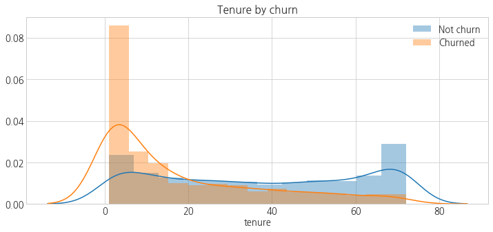
- 이탈 고객의 경우 계약 기간이 짧은 것을 확인할 수 있다.
3.5 Services & contracts
- phoneservice, multiplelines, onlinesecurity, onlinebackup, deviceprotection, techsupport, streamingtv, streamingmovies, paperlessbilling, contract(cat), internetservice(cat)
f, ax = plt.subplots(4, 3, figsize=(20, 25))
cplot(df_train, 'phoneservice', ax=ax[0,0])
cplot(df_train, 'multiplelines', ax=ax[0,1])
cplot(df_train, 'onlinesecurity', ax=ax[0,2])
cplot(df_train, 'onlinebackup', ax=ax[1,0])
cplot(df_train, 'deviceprotection', ax=ax[1,1])
cplot(df_train, 'techsupport', ax=ax[1,2])
cplot(df_train, 'streamingtv', ax=ax[2,0])
cplot(df_train, 'streamingmovies', ax=ax[2,1])
cplot(df_train, 'paperlessbilling', ax=ax[2,2])
sns.countplot('contract', data=df_train, ax=ax[3,0])
ax[3, 0].set_title('contract')
sns.countplot('internetservice', data=df_train, ax=ax[3,1])
ax[3, 1].set_title('internetservice')
sns.countplot('paymentmethod', data=df_train, ax=ax[3,2])
ax[3, 2].set_title('paymentmethod')

plt.show()
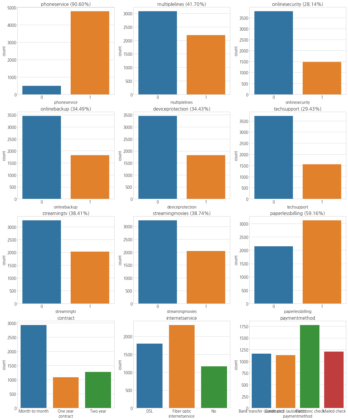
- 폰서비스를 사용하는 고객이 90% 이상이고, 그 외 서비스를 이용하는 고객들의 현황을 확인할 수 있다.
- 계약은 월별로 하는 고객이 가장 많았다.
f, ax = plt.subplots(4, 3, figsize=(20, 25))
churnplot(df_train, 'phoneservice', ax=ax[0,0])
churnplot(df_train, 'multiplelines', ax=ax[0,1])
churnplot(df_train, 'onlinesecurity', ax=ax[0,2])
churnplot(df_train, 'onlinebackup', ax=ax[1,0])
churnplot(df_train, 'deviceprotection', ax=ax[1,1])
churnplot(df_train, 'techsupport', ax=ax[1,2])
churnplot(df_train, 'streamingtv', ax=ax[2,0])
churnplot(df_train, 'streamingmovies', ax=ax[2,1])
churnplot(df_train, 'paperlessbilling', ax=ax[2,2])
sns.countplot('contract', hue='churn', data=df_train, ax=ax[3,0])
ax[3, 0].set_title('contract')
sns.countplot('internetservice', hue='churn', data=df_train, ax=ax[3,1])
ax[3, 1].set_title('internetservice')
sns.countplot('paymentmethod', hue='churn', data=df_train, ax=ax[3,2])
ax[3, 2].set_title('paymentmethod')
plt.show()
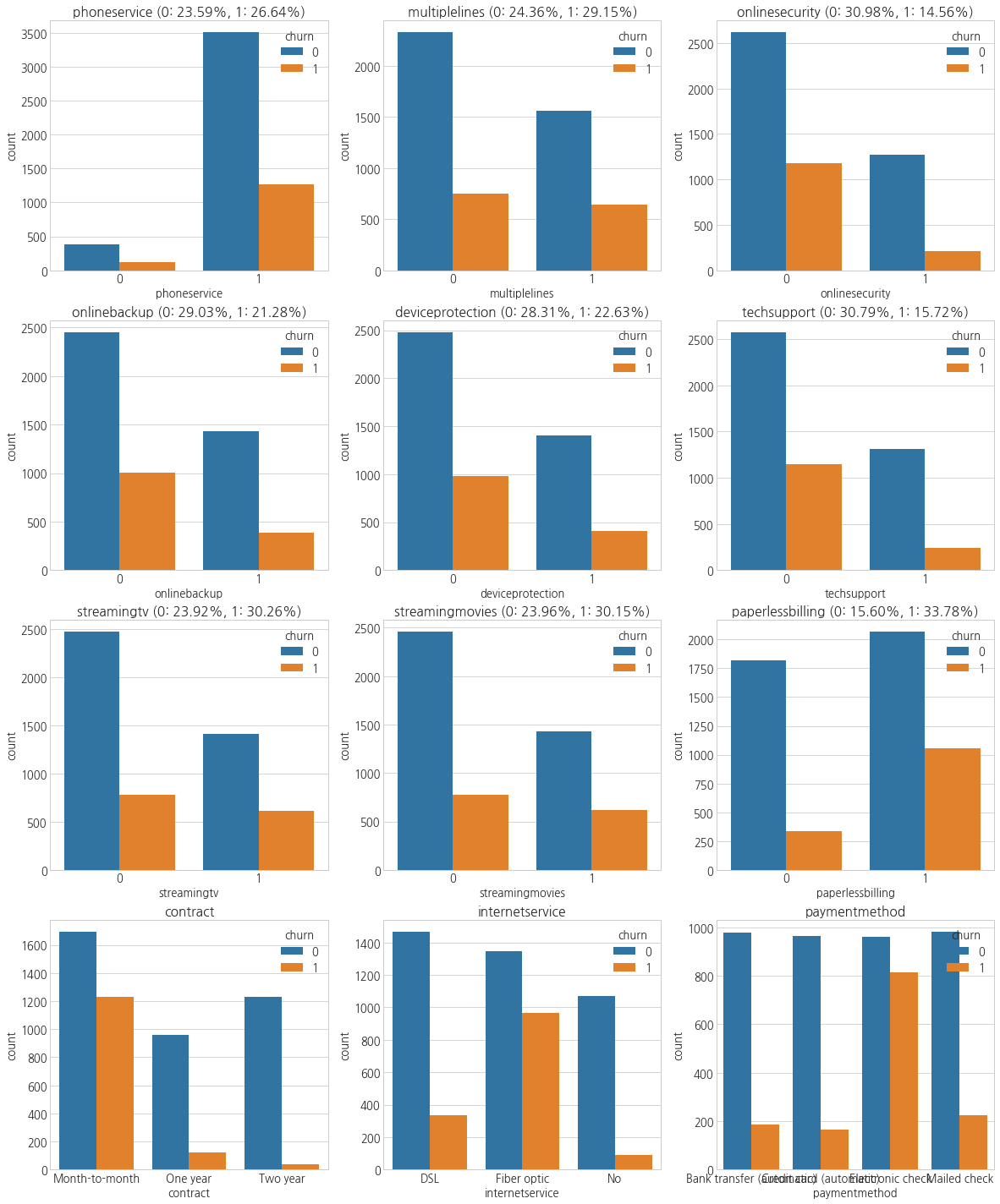
- 특이한 점은, 통지서 없이 이용하는 고객의 churnrate가 높았다.
- 그리고 월별 계약자가 가장 많았는데, churnrate 또한 세 지불 형태 중 가장 높았다.
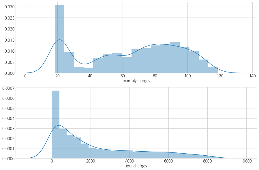
3.6 Charges
- monthlycharges, totalcharges
- 비용의 분포를 살펴보고,
- churn에 따른 비용 변화와
- 계약을 한 지 오래됐을수록 비용이 어떻게 변화하는지 함께 살펴보자.
df_train.head()
| customerid | gender | seniorcitizen | partner | dependents | tenure | phoneservice | multiplelines | internetservice | onlinesecurity | onlinebackup | deviceprotection | techsupport | streamingtv | streamingmovies | contract | paperlessbilling | paymentmethod | monthlycharges | totalcharges | churn | |
|---|---|---|---|---|---|---|---|---|---|---|---|---|---|---|---|---|---|---|---|---|---|
| 4101 | 9780-FKVVF | Male | 0 | 0 | 0 | 6 | 1 | 0 | DSL | 1 | 0 | 0 | 0 | 0 | 1 | Month-to-month | 1 | Bank transfer (automatic) | 59.15 | 336.70 | 0 |
| 3489 | 0975-UYDTX | Female | 0 | 1 | 0 | 26 | 1 | 1 | DSL | 1 | 1 | 1 | 1 | 1 | 1 | One year | 1 | Credit card (automatic) | 90.10 | 2312.55 | 0 |
| 4219 | 5176-LDKUH | Female | 0 | 0 | 0 | 48 | 1 | 0 | Fiber optic | 0 | 1 | 0 | 0 | 0 | 0 | One year | 0 | Electronic check | 75.15 | 3772.65 | 0 |
| 5091 | 2606-RMDHZ | Male | 0 | 0 | 0 | 6 | 0 | 0 | DSL | 0 | 1 | 0 | 0 | 0 | 0 | Month-to-month | 1 | Credit card (automatic) | 30.50 | 208.70 | 1 |
| 5398 | 3936-QQFLL | Male | 0 | 0 | 0 | 2 | 1 | 0 | No | 0 | 0 | 0 | 0 | 0 | 0 | Month-to-month | 0 | Mailed check | 19.75 | 39.30 | 0 |
f, ax = plt.subplots(2, 1, figsize=(15, 10))
sns.distplot(df_train.monthlycharges, ax=ax[0])
sns.distplot(df_train.totalcharges, ax=ax[1])
plt.show()
plt.figure(figsize=(7, 7))
sns.scatterplot(df_train[df_train.churn == 0].monthlycharges,
                df_train[df_train.churn == 0].totalcharges,
                label='Not churn')
sns.scatterplot(df_train[df_train.churn == 1].monthlycharges,
                df_train[df_train.churn == 1].totalcharges,
                label='Churn')
plt.show()

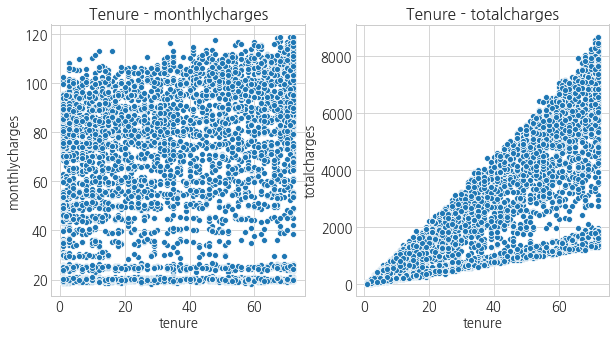
f, ax = plt.subplots(1, 2, figsize=(10, 5))
sns.scatterplot(df_train.tenure, df_train.monthlycharges, ax=ax[0])
ax[0].set_title('Tenure - monthlycharges')
sns.scatterplot(df_train.tenure, df_train.totalcharges, ax=ax[1])
ax[1].set_title('Tenure - totalcharges')
plt.show()
f, ax = plt.subplots(1, 2, figsize=(10, 5))
sns.scatterplot(df_train[df_train.churn == 0].tenure,
                df_train[df_train.churn == 0].monthlycharges, ax=ax[0],
                color='b', label='Not churn')
sns.scatterplot(df_train[df_train.churn == 1].tenure,
                df_train[df_train.churn == 1].monthlycharges, ax=ax[0],
                color='r', label='Churn')
ax[0].set_title('Tenure - monthlycharges')
sns.scatterplot(df_train[df_train.churn == 0].tenure,
                df_train[df_train.churn == 0].totalcharges, ax=ax[1],
                color='b', label='Not churn')
sns.scatterplot(df_train[df_train.churn == 1].tenure,
                df_train[df_train.churn == 1].totalcharges, ax=ax[1],
                color='r', label='Churn')
ax[1].set_title('Tenure - totalcharges')
plt.show()

- 계약 기간이 길 수록 전체 요금은 증가한다. 당연한 결과다.
- 근데, 계약 기간이 길면 각종 혜택으로 인해 월 비용이 적을 줄 알았는데, 딱히 선형관계를 보이고있지는 않다.
df_train.head()
| customerid | gender | seniorcitizen | partner | dependents | tenure | phoneservice | multiplelines | internetservice | onlinesecurity | onlinebackup | deviceprotection | techsupport | streamingtv | streamingmovies | contract | paperlessbilling | paymentmethod | monthlycharges | totalcharges | churn | |
|---|---|---|---|---|---|---|---|---|---|---|---|---|---|---|---|---|---|---|---|---|---|
| 4101 | 9780-FKVVF | Male | 0 | 0 | 0 | 6 | 1 | 0 | DSL | 1 | 0 | 0 | 0 | 0 | 1 | Month-to-month | 1 | Bank transfer (automatic) | 59.15 | 336.70 | 0 |
| 3489 | 0975-UYDTX | Female | 0 | 1 | 0 | 26 | 1 | 1 | DSL | 1 | 1 | 1 | 1 | 1 | 1 | One year | 1 | Credit card (automatic) | 90.10 | 2312.55 | 0 |
| 4219 | 5176-LDKUH | Female | 0 | 0 | 0 | 48 | 1 | 0 | Fiber optic | 0 | 1 | 0 | 0 | 0 | 0 | One year | 0 | Electronic check | 75.15 | 3772.65 | 0 |
| 5091 | 2606-RMDHZ | Male | 0 | 0 | 0 | 6 | 0 | 0 | DSL | 0 | 1 | 0 | 0 | 0 | 0 | Month-to-month | 1 | Credit card (automatic) | 30.50 | 208.70 | 1 |
| 5398 | 3936-QQFLL | Male | 0 | 0 | 0 | 2 | 1 | 0 | No | 0 | 0 | 0 | 0 | 0 | 0 | Month-to-month | 0 | Mailed check | 19.75 | 39.30 | 0 |
3.7 Correlation
- 각 컬럼간 상관 관계를 살펴보자.
df_train.head(2)
| customerid | gender | seniorcitizen | partner | dependents | tenure | phoneservice | multiplelines | internetservice | onlinesecurity | onlinebackup | deviceprotection | techsupport | streamingtv | streamingmovies | contract | paperlessbilling | paymentmethod | monthlycharges | totalcharges | churn | |
|---|---|---|---|---|---|---|---|---|---|---|---|---|---|---|---|---|---|---|---|---|---|
| 4101 | 9780-FKVVF | Male | 0 | 0 | 0 | 6 | 1 | 0 | DSL | 1 | 0 | 0 | 0 | 0 | 1 | Month-to-month | 1 | Bank transfer (automatic) | 59.15 | 336.70 | 0 |
| 3489 | 0975-UYDTX | Female | 0 | 1 | 0 | 26 | 1 | 1 | DSL | 1 | 1 | 1 | 1 | 1 | 1 | One year | 1 | Credit card (automatic) | 90.10 | 2312.55 | 0 |
plt.figure(figsize=(13, 13))
sns.heatmap(df_train.corr(), annot=True, fmt='.2f')
plt.ylim([0,21])
plt.show()

- 통신사 서비스들(streamingmovies ~ multiplelines)이 비용과 양의 상관관계가 있다.
- 또한, 서비스 이용 유무는 기간(tenure)과도 양의 상관관계를 보인다.
- 배우자 여부와 계약 기간이 양의 상관관계가 있다.
- 기간(tenure)과 churn 간 음의 상관관계가 존재한다.
4. Feature Engineering
- 일단 totalcharges와 monthlycharges, tenure를 스케일링해주자.
- 그 후 범주형 데이터를 원핫인코딩하자.
4.1 Scaling
from sklearn.preprocessing import StandardScaler
scaler = StandardScaler()
df_train[['tenure', 'monthlycharges', 'totalcharges']] =\
scaler.fit_transform(df_train[['tenure', 'monthlycharges', 'totalcharges']])
df_test[['tenure', 'monthlycharges', 'totalcharges']] =\
scaler.transform(df_test[['tenure', 'monthlycharges', 'totalcharges']])
df_train.head(3)
| customerid | gender | seniorcitizen | partner | dependents | tenure | phoneservice | multiplelines | internetservice | onlinesecurity | onlinebackup | deviceprotection | techsupport | streamingtv | streamingmovies | contract | paperlessbilling | paymentmethod | monthlycharges | totalcharges | churn | |
|---|---|---|---|---|---|---|---|---|---|---|---|---|---|---|---|---|---|---|---|---|---|
| 4101 | 9780-FKVVF | Male | 0 | 0 | 0 | -1.063702 | 1 | 0 | DSL | 1 | 0 | 0 | 0 | 0 | 1 | Month-to-month | 1 | Bank transfer (automatic) | -0.183383 | -0.850824 | 0 |
| 3489 | 0975-UYDTX | Female | 0 | 1 | 0 | -0.249401 | 1 | 1 | DSL | 1 | 1 | 1 | 1 | 1 | 1 | One year | 1 | Credit card (automatic) | 0.841167 | 0.017097 | 0 |
| 4219 | 5176-LDKUH | Female | 0 | 0 | 0 | 0.646330 | 1 | 0 | Fiber optic | 0 | 1 | 0 | 0 | 0 | 0 | One year | 0 | Electronic check | 0.346271 | 0.658466 | 0 |
4.2 One_hot_encoding
- 모델링을 위해 원핫인코딩을 진행하자.
df_train_dummy = pd.get_dummies(df_train.drop('customerid', axis=1))
df_test_dummy = pd.get_dummies(df_test.drop('customerid', axis=1))
df_train_dummy.head(2)
| seniorcitizen | partner | dependents | tenure | phoneservice | multiplelines | onlinesecurity | onlinebackup | deviceprotection | techsupport | streamingtv | streamingmovies | paperlessbilling | monthlycharges | totalcharges | churn | gender_Female | gender_Male | internetservice_DSL | internetservice_Fiber optic | internetservice_No | contract_Month-to-month | contract_One year | contract_Two year | paymentmethod_Bank transfer (automatic) | paymentmethod_Credit card (automatic) | paymentmethod_Electronic check | paymentmethod_Mailed check | |
|---|---|---|---|---|---|---|---|---|---|---|---|---|---|---|---|---|---|---|---|---|---|---|---|---|---|---|---|---|
| 4101 | 0 | 0 | 0 | -1.063702 | 1 | 0 | 1 | 0 | 0 | 0 | 0 | 1 | 1 | -0.183383 | -0.850824 | 0 | 0 | 1 | 1 | 0 | 0 | 1 | 0 | 0 | 1 | 0 | 0 | 0 |
| 3489 | 0 | 1 | 0 | -0.249401 | 1 | 1 | 1 | 1 | 1 | 1 | 1 | 1 | 1 | 0.841167 | 0.017097 | 0 | 1 | 0 | 1 | 0 | 0 | 0 | 1 | 0 | 0 | 1 | 0 | 0 |
print(df_train_dummy.shape, df_test_dummy.shape)
(5274, 28) (1758, 28)
df_train_dummy.info()
<class 'pandas.core.frame.DataFrame'>
Int64Index: 5274 entries, 4101 to 6632
Data columns (total 28 columns):
seniorcitizen                              5274 non-null int64
partner                                    5274 non-null int64
dependents                                 5274 non-null int64
tenure                                     5274 non-null float64
phoneservice                               5274 non-null int64
multiplelines                              5274 non-null int64
onlinesecurity                             5274 non-null int64
onlinebackup                               5274 non-null int64
deviceprotection                           5274 non-null int64
techsupport                                5274 non-null int64
streamingtv                                5274 non-null int64
streamingmovies                            5274 non-null int64
paperlessbilling                           5274 non-null int64
monthlycharges                             5274 non-null float64
totalcharges                               5274 non-null float64
churn                                      5274 non-null int64
gender_Female                              5274 non-null uint8
gender_Male                                5274 non-null uint8
internetservice_DSL                        5274 non-null uint8
internetservice_Fiber optic                5274 non-null uint8
internetservice_No                         5274 non-null uint8
contract_Month-to-month                    5274 non-null uint8
contract_One year                          5274 non-null uint8
contract_Two year                          5274 non-null uint8
paymentmethod_Bank transfer (automatic)    5274 non-null uint8
paymentmethod_Credit card (automatic)      5274 non-null uint8
paymentmethod_Electronic check             5274 non-null uint8
paymentmethod_Mailed check                 5274 non-null uint8
dtypes: float64(3), int64(13), uint8(12)
memory usage: 922.3 KB
df_test.info()
<class 'pandas.core.frame.DataFrame'>
Int64Index: 1758 entries, 6174 to 5663
Data columns (total 21 columns):
customerid          1758 non-null object
gender              1758 non-null object
seniorcitizen       1758 non-null int64
partner             1758 non-null int64
dependents          1758 non-null int64
tenure              1758 non-null float64
phoneservice        1758 non-null int64
multiplelines       1758 non-null int64
internetservice     1758 non-null object
onlinesecurity      1758 non-null int64
onlinebackup        1758 non-null int64
deviceprotection    1758 non-null int64
techsupport         1758 non-null int64
streamingtv         1758 non-null int64
streamingmovies     1758 non-null int64
contract            1758 non-null object
paperlessbilling    1758 non-null int64
paymentmethod       1758 non-null object
monthlycharges      1758 non-null float64
totalcharges        1758 non-null float64
churn               1758 non-null int64
dtypes: float64(3), int64(13), object(5)
memory usage: 302.2+ KB
5. Modeling
- 많은 모델들을 시도해볼 수 있겠지만, 데이터가 적고, 피처도 많은 편은 아니다.
- 또한, 이탈 고객 관련 업무는 마케팅팀, 전략팀 등과 커뮤니케이션 해야 할 일이 많을것이므로,
- Tree나 Randomforest 등 보다 비교적 설명하기 쉬운 LogisticRegressor를 사용하여 모델링을 진행해보겠다.
# 데이터 나눠주기
X_train = df_train_dummy.drop(['churn'], axis=1)
X_test = df_test_dummy.drop(['churn'], axis=1)
y_train = df_train_dummy.churn
y_test = df_test_dummy.churn
X_train.head(2)
| seniorcitizen | partner | dependents | tenure | phoneservice | multiplelines | onlinesecurity | onlinebackup | deviceprotection | techsupport | streamingtv | streamingmovies | paperlessbilling | monthlycharges | totalcharges | gender_Female | gender_Male | internetservice_DSL | internetservice_Fiber optic | internetservice_No | contract_Month-to-month | contract_One year | contract_Two year | paymentmethod_Bank transfer (automatic) | paymentmethod_Credit card (automatic) | paymentmethod_Electronic check | paymentmethod_Mailed check | |
|---|---|---|---|---|---|---|---|---|---|---|---|---|---|---|---|---|---|---|---|---|---|---|---|---|---|---|---|
| 4101 | 0 | 0 | 0 | -1.063702 | 1 | 0 | 1 | 0 | 0 | 0 | 0 | 1 | 1 | -0.183383 | -0.850824 | 0 | 1 | 1 | 0 | 0 | 1 | 0 | 0 | 1 | 0 | 0 | 0 |
| 3489 | 0 | 1 | 0 | -0.249401 | 1 | 1 | 1 | 1 | 1 | 1 | 1 | 1 | 1 | 0.841167 | 0.017097 | 1 | 0 | 1 | 0 | 0 | 0 | 1 | 0 | 0 | 1 | 0 | 0 |
5.1 측정 지표
- 측정 지표를 정하기 전에, 목적을 생각해보아야한다.
- 이탈 고객 모델링은, 이탈이라고 예측되어지는 고객에게 마케팅 메시지를 보내어 이탈을 방지하는 것이 목적이다.
- 그러므로, 실제 이탈 고객을 얼마나 많이 찾아내는가가 중요하다.
- 따라서, 재현율(recall), f1score를 지표로 사용해보겠다.
5.2 Baseline
- 튜닝 없이 바로 모델에 넣어서 성능을 확인해보자.
from sklearn.linear_model import LogisticRegression
from sklearn.metrics import recall_score, precision_score, f1_score

logreg = LogisticRegression()
logreg.fit(X_train, y_train)
y_pred = logreg.predict(X_train)
def print_score(y_true, y_pred):
    print('recall: {:.2f}\nprecision: {:.2f}\nf1_score: {:.2f}'.format(
        recall_score(y_true, y_pred), precision_score(y_true, y_pred), f1_score(y_true, y_pred)))
print_score(y_train, y_pred)
recall: 0.55
precision: 0.67
f1_score: 0.61
- 재현율이 55%밖에 되지 않는다.
- 나머지 45%에 대한 실제값은 잃게되고, 모델의 본 목적을 이루지 못할 수 있다.
- confusion matrix를 나타내보자.
from sklearn.metrics import confusion_matrix
confusion_matrix(y_train, y_pred)
array([[3512,  372],
       [ 621,  769]], dtype=int64)
- Negative에 대해서는 나름 성능이 좋은데, Positive에 대해서는 예측력이 떨어진다.
- test세트에선 어떻게 나타나는지 살펴보자.
y_pred = logreg.predict(X_test)
recall_score(y_test, y_pred)
0.5407098121085595
- 테스트 세트에서도 당연히 좋지 않은 성능을 보이고 있다.
- Feature Selection을 통해 중요도가 낮은 특성을 제외시켜보자.
5.3 Feature Selection
- 피처 선택 방법엔 많은 방법이 있지만, RandomForest에서 제공하는 feature_importance_를 통해 진행해보자.
from sklearn.ensemble import RandomForestClassifier
rf = RandomForestClassifier(n_estimators=500, max_depth=8, random_state=1)
rf.fit(X_train, y_train)
df_fi = pd.DataFrame(rf.feature_importances_, index=X_train.columns, columns=['importances'])
df_fi.sort_values('importances', ascending=True, inplace=True)
df_fi.plot(kind='barh', figsize=(10,10))
<matplotlib.axes._subplots.AxesSubplot at 0x114ef310688>

- 각종 부가 서비스들(phoneservice, onlinebackup, streamingtv 등)의 중요도가 낮다.
- 또한, 성별과 자녀, 배우자 등 인구통계학적 정보들도 중요도가 낮다.
- 0.02 이하인 특성들을 제거해보자.
col_selected = list(df_fi[df_fi.importances>=0.02].index)
col_selected
['internetservice_DSL',
 'paperlessbilling',
 'internetservice_No',
 'contract_Two year',
 'paymentmethod_Electronic check',
 'internetservice_Fiber optic',
 'monthlycharges',
 'totalcharges',
 'contract_Month-to-month',
 'tenure']
- 이제 이 특성들만 남기고 다시 모델링을 진행해보자.
X_train_selected = X_train[col_selected]
X_test_selected = X_test[col_selected]

logreg = LogisticRegression()
logreg.fit(X_train_selected, y_train)
y_pred = logreg.predict(X_train_selected)

print_score(y_train, y_pred)
recall: 0.53
precision: 0.66
f1_score: 0.59
- 불필요한 특성들을 제거하니 오히려 성능이 떨어졌다.
- 이번에는 lable의 가중치와 C값을 변화시켜 성능을 올려보자.
5.4 Class_wight, C
- Churn의 0과 1의 비율은 약 7.5:2.5 였다.
- 이를 반영하여 모델에 적용시켜서 성능을 확인해보자.
logreg = LogisticRegression(class_weight={0: 0.25, 1: 0.75})
logreg.fit(X_train_selected, y_train)
y_pred = logreg.predict(X_train_selected)
print_score(y_train, y_pred)
confusion_matrix(y_train, y_pred)
recall: 0.83
precision: 0.50
f1_score: 0.62


array([[2719, 1165],
       [ 238, 1152]], dtype=int64)
- 재현율이 확실히 높아졌다! 하지만 그만큼 정밀도는 전에 비해 하락하였다.
- 이번에는 C값을 조정하여 성능을 올려보자.
logreg = LogisticRegression(C=0.001, class_weight={0: 0.25, 1: 0.75})
logreg.fit(X_train_selected, y_train)
y_pred = logreg.predict(X_train_selected)
print_score(y_train, y_pred)
confusion_matrix(y_train, y_pred)
recall: 0.89
precision: 0.42
f1_score: 0.57


array([[2182, 1702],
       [ 152, 1238]], dtype=int64)
- 모델에 규제를 적용하니, 재현율은 0.89로 높아지나, 정밀도와 f1점수가 낮아진다.
5.5 GridSearch
- 그리드서치를 통해 최적의 C, Class_weight 값을 찾아보자.
from sklearn.model_selection import GridSearchCV
param_grid = {'C': [1000, 100, 10, 1, 0.1, 0.01, 0.001, 0.0001],
              'class_weight': [{0: 0.2, 1: 0.8}, {0: 0.25, 1: 0.75},{0: 0.3, 1: 0.7},{0: 0.35, 1: 0.65}]}
grid_search = GridSearchCV(LogisticRegression(), param_grid=param_grid, scoring='f1')
grid_search.fit(X_train_selected, y_train)
GridSearchCV(cv='warn', error_score='raise-deprecating',
             estimator=LogisticRegression(C=1.0, class_weight=None, dual=False,
                                          fit_intercept=True,
                                          intercept_scaling=1, l1_ratio=None,
                                          max_iter=100, multi_class='warn',
                                          n_jobs=None, penalty='l2',
                                          random_state=None, solver='warn',
                                          tol=0.0001, verbose=0,
                                          warm_start=False),
             iid='warn', n_jobs=None,
             param_grid={'C': [1000, 100, 10, 1, 0.1, 0.01, 0.001, 0.0001],
                         'class_weight': [{0: 0.2, 1: 0.8}, {0: 0.25, 1: 0.75},
                                          {0: 0.3, 1: 0.7},
                                          {0: 0.35, 1: 0.65}]},
             pre_dispatch='2*n_jobs', refit=True, return_train_score=False,
             scoring='f1', verbose=0)
pd.DataFrame(grid_search.cv_results_).sort_values('rank_test_score')
| mean_fit_time | std_fit_time | mean_score_time | std_score_time | param_C | param_class_weight | params | split0_test_score | split1_test_score | split2_test_score | mean_test_score | std_test_score | rank_test_score | |
|---|---|---|---|---|---|---|---|---|---|---|---|---|---|
| 15 | 0.013962 | 0.000815 | 0.004322 | 1.244091e-03 | 1 | {0: 0.35, 1: 0.65} | {'C': 1, 'class_weight': {0: 0.35, 1: 0.65}} | 0.612903 | 0.667921 | 0.613746 | 0.631523 | 0.025739 | 1 |
| 3 | 0.017204 | 0.004256 | 0.001995 | 1.410627e-03 | 1000 | {0: 0.35, 1: 0.65} | {'C': 1000, 'class_weight': {0: 0.35, 1: 0.65}} | 0.615385 | 0.664799 | 0.613308 | 0.631164 | 0.023799 | 2 |
| 7 | 0.016290 | 0.003389 | 0.004987 | 8.163403e-04 | 100 | {0: 0.35, 1: 0.65} | {'C': 100, 'class_weight': {0: 0.35, 1: 0.65}} | 0.615385 | 0.664799 | 0.613308 | 0.631164 | 0.023799 | 2 |
| 11 | 0.013297 | 0.001245 | 0.003990 | 8.143937e-04 | 10 | {0: 0.35, 1: 0.65} | {'C': 10, 'class_weight': {0: 0.35, 1: 0.65}} | 0.615385 | 0.666043 | 0.611969 | 0.631133 | 0.024725 | 4 |
| 10 | 0.015956 | 0.001411 | 0.003325 | 4.697983e-04 | 10 | {0: 0.3, 1: 0.7} | {'C': 10, 'class_weight': {0: 0.3, 1: 0.7}} | 0.616207 | 0.653584 | 0.615794 | 0.628528 | 0.017718 | 5 |
| 2 | 0.011807 | 0.001018 | 0.002327 | 1.694859e-03 | 1000 | {0: 0.3, 1: 0.7} | {'C': 1000, 'class_weight': {0: 0.3, 1: 0.7}} | 0.614973 | 0.654142 | 0.614703 | 0.627939 | 0.018528 | 6 |
| 6 | 0.013641 | 0.001710 | 0.004643 | 1.232730e-03 | 100 | {0: 0.3, 1: 0.7} | {'C': 100, 'class_weight': {0: 0.3, 1: 0.7}} | 0.614973 | 0.654142 | 0.614703 | 0.627939 | 0.018528 | 6 |
| 14 | 0.014959 | 0.000815 | 0.004655 | 1.244580e-03 | 1 | {0: 0.3, 1: 0.7} | {'C': 1, 'class_weight': {0: 0.3, 1: 0.7}} | 0.620321 | 0.648464 | 0.611807 | 0.626866 | 0.015663 | 8 |
| 18 | 0.012633 | 0.000940 | 0.003323 | 4.700783e-04 | 0.1 | {0: 0.3, 1: 0.7} | {'C': 0.1, 'class_weight': {0: 0.3, 1: 0.7}} | 0.623214 | 0.650477 | 0.606278 | 0.626660 | 0.018205 | 9 |
| 22 | 0.013629 | 0.000940 | 0.004656 | 4.687292e-04 | 0.01 | {0: 0.3, 1: 0.7} | {'C': 0.01, 'class_weight': {0: 0.3, 1: 0.7}} | 0.611599 | 0.643894 | 0.605846 | 0.620448 | 0.016745 | 10 |
| 19 | 0.013630 | 0.003084 | 0.003657 | 4.711456e-04 | 0.1 | {0: 0.35, 1: 0.65} | {'C': 0.1, 'class_weight': {0: 0.35, 1: 0.65}} | 0.607280 | 0.653956 | 0.596421 | 0.619221 | 0.024958 | 11 |
| 13 | 0.014960 | 0.000815 | 0.003991 | 2.734606e-06 | 1 | {0: 0.25, 1: 0.75} | {'C': 1, 'class_weight': {0: 0.25, 1: 0.75}} | 0.611339 | 0.636148 | 0.605154 | 0.617548 | 0.013392 | 12 |
| 9 | 0.013629 | 0.000940 | 0.004324 | 4.704158e-04 | 10 | {0: 0.25, 1: 0.75} | {'C': 10, 'class_weight': {0: 0.25, 1: 0.75}} | 0.609053 | 0.636148 | 0.604149 | 0.616451 | 0.014071 | 13 |
| 5 | 0.013297 | 0.000471 | 0.003991 | 8.143941e-04 | 100 | {0: 0.25, 1: 0.75} | {'C': 100, 'class_weight': {0: 0.25, 1: 0.75}} | 0.608553 | 0.635071 | 0.603648 | 0.615758 | 0.013802 | 14 |
| 1 | 0.017287 | 0.002349 | 0.005651 | 1.243349e-03 | 1000 | {0: 0.25, 1: 0.75} | {'C': 1000, 'class_weight': {0: 0.25, 1: 0.75}} | 0.608553 | 0.635071 | 0.603648 | 0.615758 | 0.013802 | 14 |
| 17 | 0.012965 | 0.001410 | 0.004322 | 4.694603e-04 | 0.1 | {0: 0.25, 1: 0.75} | {'C': 0.1, 'class_weight': {0: 0.25, 1: 0.75}} | 0.608553 | 0.633333 | 0.602831 | 0.614907 | 0.013237 | 16 |
| 23 | 0.013962 | 0.000815 | 0.006317 | 1.696106e-03 | 0.01 | {0: 0.35, 1: 0.65} | {'C': 0.01, 'class_weight': {0: 0.35, 1: 0.65}} | 0.606635 | 0.633962 | 0.584403 | 0.608338 | 0.020266 | 17 |
| 27 | 0.008312 | 0.000940 | 0.005563 | 1.227498e-03 | 0.001 | {0: 0.35, 1: 0.65} | {'C': 0.001, 'class_weight': {0: 0.35, 1: 0.65}} | 0.595822 | 0.636861 | 0.592251 | 0.608312 | 0.020240 | 18 |
| 21 | 0.012633 | 0.000949 | 0.006645 | 1.690214e-03 | 0.01 | {0: 0.25, 1: 0.75} | {'C': 0.01, 'class_weight': {0: 0.25, 1: 0.75}} | 0.595444 | 0.622188 | 0.598879 | 0.605503 | 0.011881 | 19 |
| 8 | 0.015292 | 0.001243 | 0.003989 | 8.136148e-04 | 10 | {0: 0.2, 1: 0.8} | {'C': 10, 'class_weight': {0: 0.2, 1: 0.8}} | 0.597084 | 0.610465 | 0.599847 | 0.602465 | 0.005769 | 20 |
| 0 | 0.015626 | 0.000468 | 0.004653 | 4.706434e-04 | 1000 | {0: 0.2, 1: 0.8} | {'C': 1000, 'class_weight': {0: 0.2, 1: 0.8}} | 0.596923 | 0.610022 | 0.599847 | 0.602263 | 0.005614 | 21 |
| 4 | 0.013168 | 0.000288 | 0.003325 | 4.699655e-04 | 100 | {0: 0.2, 1: 0.8} | {'C': 100, 'class_weight': {0: 0.2, 1: 0.8}} | 0.596923 | 0.610022 | 0.599847 | 0.602263 | 0.005614 | 21 |
| 12 | 0.012965 | 0.000814 | 0.004321 | 4.714266e-04 | 1 | {0: 0.2, 1: 0.8} | {'C': 1, 'class_weight': {0: 0.2, 1: 0.8}} | 0.596330 | 0.609579 | 0.599085 | 0.601664 | 0.005708 | 23 |
| 31 | 0.008644 | 0.001245 | 0.003324 | 4.699096e-04 | 0.0001 | {0: 0.35, 1: 0.65} | {'C': 0.0001, 'class_weight': {0: 0.35, 1: 0.65}} | 0.583129 | 0.623509 | 0.596939 | 0.601190 | 0.016759 | 24 |
| 16 | 0.012634 | 0.000941 | 0.003656 | 9.407739e-04 | 0.1 | {0: 0.2, 1: 0.8} | {'C': 0.1, 'class_weight': {0: 0.2, 1: 0.8}} | 0.584151 | 0.611354 | 0.596651 | 0.597383 | 0.011119 | 25 |
| 26 | 0.011967 | 0.000813 | 0.003989 | 8.146874e-04 | 0.001 | {0: 0.3, 1: 0.7} | {'C': 0.001, 'class_weight': {0: 0.3, 1: 0.7}} | 0.578078 | 0.607768 | 0.592366 | 0.592735 | 0.012126 | 26 |
| 20 | 0.011303 | 0.000941 | 0.002991 | 7.867412e-07 | 0.01 | {0: 0.2, 1: 0.8} | {'C': 0.01, 'class_weight': {0: 0.2, 1: 0.8}} | 0.566690 | 0.581619 | 0.582511 | 0.576937 | 0.007258 | 27 |
| 30 | 0.007978 | 0.000002 | 0.003656 | 9.409429e-04 | 0.0001 | {0: 0.3, 1: 0.7} | {'C': 0.0001, 'class_weight': {0: 0.3, 1: 0.7}} | 0.553672 | 0.584462 | 0.578871 | 0.572330 | 0.013395 | 28 |
| 25 | 0.010970 | 0.000816 | 0.004654 | 4.683920e-04 | 0.001 | {0: 0.25, 1: 0.75} | {'C': 0.001, 'class_weight': {0: 0.25, 1: 0.75}} | 0.549598 | 0.573925 | 0.569855 | 0.564456 | 0.010641 | 29 |
| 29 | 0.010136 | 0.005132 | 0.002660 | 1.880649e-03 | 0.0001 | {0: 0.25, 1: 0.75} | {'C': 0.0001, 'class_weight': {0: 0.25, 1: 0.75}} | 0.527445 | 0.548896 | 0.543590 | 0.539974 | 0.009124 | 30 |
| 24 | 0.010971 | 0.000813 | 0.004322 | 4.703590e-04 | 0.001 | {0: 0.2, 1: 0.8} | {'C': 0.001, 'class_weight': {0: 0.2, 1: 0.8}} | 0.529557 | 0.539818 | 0.543071 | 0.537479 | 0.005760 | 31 |
| 28 | 0.008310 | 0.000471 | 0.003990 | 8.152695e-04 | 0.0001 | {0: 0.2, 1: 0.8} | {'C': 0.0001, 'class_weight': {0: 0.2, 1: 0.8}} | 0.506344 | 0.511761 | 0.521077 | 0.513058 | 0.006084 | 32 |
grid_search.best_params_
{'C': 1, 'class_weight': {0: 0.35, 1: 0.65}}
- 최적의 파라미터를 찾았으니, 이 파라미터로 모델을 훈련시켜보자.
logreg = LogisticRegression(C=1, class_weight={0: 0.35, 1: 0.65})
logreg.fit(X_train_selected, y_train)
y_pred = logreg.predict(X_train_selected)
print_score(y_train, y_pred)
confusion_matrix(y_train, y_pred)
recall: 0.72
precision: 0.57
f1_score: 0.64


array([[3118,  766],
       [ 386, 1004]], dtype=int64)
- 재현율은 baseline인 0.55보다 개선되었다.
- 재현율과 트레이드오프 관계에 있는 정밀도는 기존보다 떨어졌다.
- 이 모델이 test세트에는 잘 작동하는지 살펴보자.
y_pred = logreg.predict(X_test_selected)
print_score(y_test, y_pred)
confusion_matrix(y_test, y_pred)
recall: 0.69
precision: 0.55
f1_score: 0.61


array([[1014,  265],
       [ 150,  329]], dtype=int64)
- 재현율이 0.69로 나온다.
- 그리드서치로 튜닝이 많이 된 모델의 경우, 일반적으로 테스트세트에선 지표가 낮게 나온다고 한다.
- 또한, 여기서 성능을 더 올리기 위해 튜닝을 추가로 하지는 않는다고 한다.
- (핸즈온 머신러닝 책에서)
- 실제의 이탈 고객을 약 69% 예측할 수 있는 모델을 만드는데에 성공했다.
6. 비즈니스에 적용해본다면?
이 모델을 어떻게 적용할 수 있을까? 간단하게 생각해보자.
- 특성 중 요금이 모델링에 중요한 영향을 끼쳤으므로, 가격 정책에 대해 검토해본다.
- 이탈 예정이라고 예측된 고객에게 현재 사용하고 있는 서비스에 만족하는지에 대해 조사해본다.
- 개선이 가능한 점이 있다면 개선하고, 요금의 문제라면 이탈할 것이라고 예측되는 고객에 대해 요금 할인 정책을 진행해본다.
- 통신사에 대해선 도메인 지식이 부족해서 이 정도 아이디어밖에 떠오르지가 않는다…
서비스가 커머스라고 가정하면,
- 이탈 예정 고객을 예측한다.
- 예측된 고객이 어떤 특징을 갖고 있는지, 그리고 최근에 이용한 서비스는 무엇인지, 행태는 어떤지 분석한다.
- 브랜드가 전달하고자하는 메시지가 고객에게 잘 전달되고있는지도 확인한다.
- 그리고 고객과 커뮤니케이션이 잘 되고 있는지도 확인해본다. (고객이 우리의 소식을 잘 받고 계신지)
- 가격이 원인이었다면, 예측된 고객에게 할인 쿠폰이나, 서비스 무료 이용권 등을 배포해본다.
- 설문조사를 실시해서 어떤 부분이 마음에 들지 않았는지 확인해본다.
- 위와 동일하게, 개선이 가능한 부분이 있다면 개선해본다.
- 그들이 실제로 이탈하지 않고 지속되고있는지 모니터링한다.
- 지속적으로 유지보수하고 개선해나간다…
6.1 현업에선..
- 운이 좋지 않은 이상, 이렇게 정제가 잘 되어있는 1차 데이터가 존재하지 않는다.
- 그리고 어떤 특성들을 1차로 선택할 지 도메인지식이 많이 필요할것이다.
- 그럼에도 고객데이터가 churn으로 나뉜 오픈 데이터셋은 많지 않아서 통신사 데이터를 활용하여 예측 모델을 만들어보았다.
- 확실히 도메인지식이 부족해서 데이터를 이해함에 있어서 어려움이 있었지만,
- 커머스 데이터에는 어떻게 적용할 수 있을지에 대해 고민하며 진행하다보니, 재미있게 할 수 있었다.
- 실제 현업에서는 이런 분석들을 어떻게 고도화하여 진행하는지 궁금하고, 기여해보고싶다.
댓글남기기